Data Wrangling with tidyr
Last updated on 2026-06-30 | Edit this page
Estimated time: 40 minutes
- The primary goal is to help learners understand how to clean their data and change table formats for different uses.
- Similarly to Data Wrangling with dplyr, this lesson works better if you can use graphics to demonstrate the difference between long and wide table formats. We have created this Google Slides deck for this purpose!
Overview
Questions
- How can I reformat a tibble to meet my needs?
Objectives
- Describe the concept of a wide and a long table format and for which purpose those formats are useful.
- Describe the roles of variable names and their associated values when a table is reshaped.
- Reshape a tibble from long to wide format and back with the
pivot_widerandpivot_longercommands from thetidyrpackage.
dplyr pairs nicely with
tidyr, a package that enables you to
swiftly convert between different data formats (long vs. wide) for
plotting and analysis. To learn more about
tidyr after the workshop, you may want to
check out this handy
data tidying with tidyr
cheatsheet.
To make sure everyone will use the same data sets for this lesson, we’ll be reading in the updated version of the Check-In Dataset (as created in “Starting With Data”), as well as the Messy Dataset (which we will cover at the end of this lesson).
Reading in Data
To start, we will load in the tidyverse
and here packages so we can read in our
CSV files.
R
library(tidyverse)
library(here)
Next, we will read in the Check-In Data:
R
data <- read_csv(here("data", "checkin_data_2.csv"))
Reshaping with pivot_wider() and pivot_longer()
There are essentially three rules that define a “tidy” data set:
- Each variable has its own column
- Each observation has its own row
- Each value must have its own cell
This graphic visually represents the three rules that define a “tidy” data set:
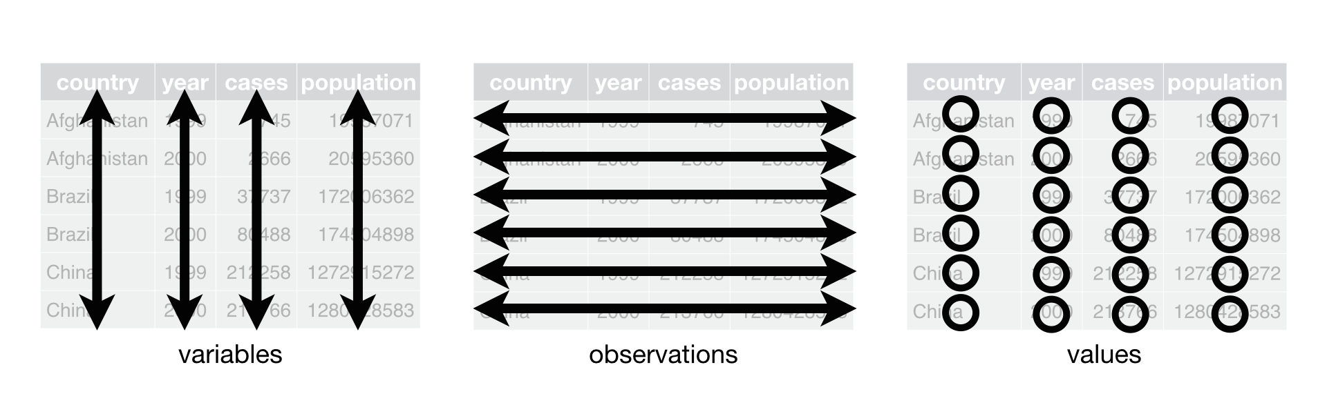 R for Data Science, Wickham H and Grolemund G (https://r4ds.had.co.nz/index.html)
© Wickham, Grolemund 2017 This image is licensed under
Attribution-NonCommercial-NoDerivs 3.0 United States (CC-BY-NC-ND 3.0
US)
R for Data Science, Wickham H and Grolemund G (https://r4ds.had.co.nz/index.html)
© Wickham, Grolemund 2017 This image is licensed under
Attribution-NonCommercial-NoDerivs 3.0 United States (CC-BY-NC-ND 3.0
US)
In this section we will explore how these rules are linked to the different data formats researchers are often interested in: “wide” and “long”. This tutorial will help you efficiently transform your data shape, regardless of its original format.
First, we will explore qualities of the data data and
how they relate to these different types of data formats.
Long and Wide Data Formats
In data, each row contains the values of variables
associated with each record collected (each ballot instance). As you may
recall from “Starting With Data”, it was stated that the
checkin_id was added to provide a “unique key/ID” for each
individual ballot.
Since checkin_id is unique to each instance, we can use
this variable as an identifier corresponding to each of the 352112
observations.
R
data %>%
  select(checkin_id) %>%
  distinct() %>%
  nrow()
OUTPUT
[1] 352112As seen in the code below, for each check-in time corresponding to
each device, no two checkin_ids are the same. Thus, this
format is what we call a “long” data format, where each observation
occupies only one row in the tibble.
R
data %>%
  filter(location == "LOCATION_001") %>%
  select(checkin_id, checkin_time, location) %>%
  sample_n(size = 10)
OUTPUT
# A tibble: 10 × 3
   checkin_id     checkin_time        location
   <chr>          <dttm>              <chr>
 1 CHECKIN_000067 2018-11-06 08:12:23 LOCATION_001
 2 CHECKIN_000075 2018-11-06 08:19:08 LOCATION_001
 3 CHECKIN_000266 2018-11-06 11:03:23 LOCATION_001
 4 CHECKIN_000536 2018-11-06 17:33:14 LOCATION_001
 5 CHECKIN_000159 2018-11-06 09:28:50 LOCATION_001
 6 CHECKIN_000274 2018-11-06 11:16:58 LOCATION_001
 7 CHECKIN_000320 2018-11-06 11:52:43 LOCATION_001
 8 CHECKIN_000167 2018-11-06 09:34:43 LOCATION_001
 9 CHECKIN_000388 2018-11-06 13:42:07 LOCATION_001
10 CHECKIN_000393 2018-11-06 13:49:08 LOCATION_001
If you were to look at the entire data data set, you
would notice that the layout/format of the data adheres to rules 1-3,
where:
- each column is a variable
- each row is an observation
- each value has its own cell
As mentioned above, this is called a “long” data format. Additionally, you may notice that each column represents a different variable. In the “longest” data format there would only be three columns, one for the id variable, one for the observed variable, and one for the observed value (of that variable). This data format is quite unsightly and difficult to work with, so you will rarely see it in use.
Alternatively, in a “wide” data format we see modifications to rule 1, where each column no longer represents a single variable. Instead, columns can represent different levels/values of a variable. For instance, in some data you encounter, the researchers may have chosen for every check-in hour to be a different column.
These may sound like dramatically different data layouts, but there are some tools that make transitions between these layouts much simpler than you might think! The GIF below shows how these two formats relate to each other, and gives you an idea of how we can use R to shift from one format to the other.
Long and wide tibble layouts mainly affect readability. You may find that visually you may prefer the “wide” format, since you can see more of the data on the screen. However, all of the R functions we have used thus far expect for your data to be in a “long” data format. This is because the long format is more machine readable and is closer to the formatting of databases.
Questions That Warrant Different Data Formats
In data, each row contains values associated with each
record (the unit). This may include values such as the ID of the ballot
box, the ballot box’s location, the precinct the ballot box belongs to,
or the arrival time of the person submitting the ballot. This format
allows for us to make comparisons across individual ballot
instances!
However, what if we wanted to look at how many check-ins occurred each hour in regards to each polling location?
To facilitate this comparison, we would need to create a new table
where each row (the unit) represents a polling location (associated with
the location column), each column (after the first)
represents an hour of the day (associated with the hour
column), and the values of each row containing the number of check-ins
recorded at that location during that hour.
Once we we’ve created this new table, we can explore the relationships within and between locations. The key point here is that we are still following a tidy data structure, but we have reshaped the data according to the observations of interest.
Alternatively, let’s say the check-in times were originally spread across multiple columns, and we were interested in visualizing, across multiple locations, how check-in activity has changed over the course of the day. This would require the check-in time to be included in a single column rather than spread across multiple columns. Thus, we would need to transform the column names into the values of a variable.
We can do both of these transformations with two
tidyr functions,
pivot_wider() and pivot_longer().
Pivoting Wider
pivot_wider() takes in three principal arguments:
- the data to be transformed
- the names_from column variable (whose values will become new column names).
- the values_from column variable (whose values will fill the new column variables).
Further arguments include values_fill which, if set,
fills in missing values with the value provided, and
names_sort, which, if set, sorts the columns in
alphanumerical order.
Let’s use pivot_wider() to transform data
to create new columns for each hour represented within the data.
To help with understanding, we will be walking through the transformation line-by-line.
First we create a new object (data_tc) based on the
data tibble:
Our next step will be to get the values for each cell, so we will be
using the count() function from the
dplyr package. This is completed in the
next line, grouping by location and hour:
Finally, we will be creating and populating the new, “wide” data using the counts and the column values! This can be seen below:
R
pivot_wider(
  names_from = hour,
  values_from = n,
  values_fill = 0
)
Now that we understand what’s going on, let’s combine all those chunks together and look at what our completed tibble looks like!
R
#create the object
data_tc <- data %>%
  #get the values
  count(location, hour) %>%
  #pivot the data
  pivot_wider(
  names_from = hour,
  values_from = n,
  values_fill = 0
)

head(data_tc)
OUTPUT
# A tibble: 6 × 16
  location       `7`   `8`   `9`  `10`  `11`  `12`  `13`  `14`  `15`  `16`  `17`
  <chr>        <int> <int> <int> <int> <int> <int> <int> <int> <int> <int> <int>
1 LOCATION_001    50    71    77    62    65    40    41    30    28    35    62
2 LOCATION_002    16    29    19    32    14    22    14    13    19    20    24
3 LOCATION_003    74    69    88   106    65    64    54    42    49    51    55
4 LOCATION_004    81    74    73    61    59    29    35    36    42    45    54
5 LOCATION_005    53    31    57    64    61    49    57    45    54    67    99
6 LOCATION_006   115    65    75    75    78    44    50    52    50    92    88
# ℹ 4 more variables: `18` <int>, `19` <int>, `6` <int>, `20` <int>
Oh no! It looks like the hours columns are out of order, with 6 sitting between 19 and 20. If we were to perform data analysis, this would not matter, but visually, this can be confusing or misleading, since we expect time to move from left to right in ascending order.
In order to fix this, we can add the aforementioned
names_sort argument to the function to specify that the
columns should be in order. This line has been added to the code block
below:
R
#create the object
data_tc <- data %>%
  #get the values
  count(location, hour) %>%
  #pivot the data
  pivot_wider(
  names_from = hour,
  values_from = n,
  values_fill = 0,
  names_sort = TRUE #sorts the columns from left to right
)

head(data_tc)
OUTPUT
# A tibble: 6 × 16
  location       `6`   `7`   `8`   `9`  `10`  `11`  `12`  `13`  `14`  `15`  `16`
  <chr>        <int> <int> <int> <int> <int> <int> <int> <int> <int> <int> <int>
1 LOCATION_001     0    50    71    77    62    65    40    41    30    28    35
2 LOCATION_002     0    16    29    19    32    14    22    14    13    19    20
3 LOCATION_003     0    74    69    88   106    65    64    54    42    49    51
4 LOCATION_004     0    81    74    73    61    59    29    35    36    42    45
5 LOCATION_005     0    53    31    57    64    61    49    57    45    54    67
6 LOCATION_006     1   115    65    75    75    78    44    50    52    50    92
# ℹ 4 more variables: `17` <int>, `18` <int>, `19` <int>, `20` <int>
As seen by the outputted tibble above, the hour columns now appear in ascending order, making the table far easier to interpret at a glance!
Now that we’ve used pivot_wider() to make our data
“wide”, let’s take a closer look at the resulting data_tc
tibble to gain a better understanding.
First, let’s check the dimensions:
R
dim(data_tc)
OUTPUT
[1] 417 16As we can see, there are 417 rows and 16 columns! Each row represents
a unique location within the data set. We can verify this by counting
the number of unique location values within data:
R
n_distinct(data$location)
OUTPUT
[1] 417This also returns 417, confirming that each row corresponds to a single, unique location within the data.
Next, let’s look at the 16 columns of the tibble:
R
colnames(data_tc)
OUTPUT
 [1] "location" "6"        "7"        "8"        "9"        "10"
 [7] "11"       "12"       "13"       "14"       "15"       "16"
[13] "17"       "18"       "19"       "20"
Notice there is no longer a column titled hour. This is
because the pivot_wider() function, by default, removes the
original column that the new column values were taken from. In this
case, the values from the original hour column have now
become columns with names that range from 6 to 20, representing the
hours from 6AM to 8PM, and thus the hour column has been
dropped.
This new format of the data allows us to do interesting things, like make a table showing the number of check-ins across all locations at a particular time, with the rows being ordered from highest to lowest in terms of count:
R
data_tc %>%
  select(location, `7`) %>%
  arrange(desc(`7`))
OUTPUT
# A tibble: 417 × 2
   location       `7`
   <chr>        <int>
 1 LOCATION_233   234
 2 LOCATION_364   215
 3 LOCATION_258   212
 4 LOCATION_366   197
 5 LOCATION_417   197
 6 LOCATION_306   194
 7 LOCATION_317   193
 8 LOCATION_166   189
 9 LOCATION_403   188
10 LOCATION_386   183
# ℹ 407 more rows
Or, we can calculate the total amount of check-ins for each location across all hours, and sort the data to determine which location had the least check-ins:
R
data_tc %>%
  mutate(total_checkins = rowSums(data_tc[-1])) %>%
  select(location, total_checkins) %>%
  arrange(total_checkins)
OUTPUT
# A tibble: 417 × 2
   location     total_checkins
   <chr>                 <dbl>
 1 LOCATION_048              2
 2 LOCATION_308             11
 3 LOCATION_393             38
 4 LOCATION_103             42
 5 LOCATION_280             42
 6 LOCATION_164             58
 7 LOCATION_298             60
 8 LOCATION_101             64
 9 LOCATION_014             66
10 LOCATION_138             68
# ℹ 407 more rowsExercise
We created data_tc by reshaping the data. Replicate this
process to create a tibble named data_total that shows the
total number of check-ins for each hour, across all locations.
The resulting tibble should have columns for each hour, sorted from
earliest to latest similarly to the data_tc tibble. There
should only be one row, representative of all locations, and an extra
summary column, called total_checkins, that calculates the
total number of check ins across the entire data data
set.
R
data_total <- data %>%
  count(hour) %>%
  pivot_wider(
    names_from = hour,
    values_from = n,
    values_fill = 0,
    names_sort = TRUE
    ) %>%
  mutate(total_checkins = rowSums(across(everything())))

data_total
OUTPUT
# A tibble: 1 × 16
    `6`   `7`   `8`   `9`  `10`  `11`  `12`  `13`  `14`  `15`  `16`  `17`  `18`
  <int> <int> <int> <int> <int> <int> <int> <int> <int> <int> <int> <int> <int>
1   265 34918 29613 34076 35186 30909 23119 21751 20178 23233 28925 31774 25924
# ℹ 3 more variables: `19` <int>, `20` <int>, total_checkins <dbl>
R
#alternative solution:
data_total_2 <- data %>%
  count(hour) %>%
  pivot_wider(
    names_from = hour,
    values_from = n,
    values_fill = 0,
    names_sort = TRUE
    )

data_total_2 <- data_total_2 %>%
  mutate(total_checkins = rowSums(data_total_2))

data_total_2
OUTPUT
# A tibble: 1 × 16
    `6`   `7`   `8`   `9`  `10`  `11`  `12`  `13`  `14`  `15`  `16`  `17`  `18`
  <int> <int> <int> <int> <int> <int> <int> <int> <int> <int> <int> <int> <int>
1   265 34918 29613 34076 35186 30909 23119 21751 20178 23233 28925 31774 25924
# ℹ 3 more variables: `19` <int>, `20` <int>, total_checkins <dbl>
Pivoting Longer
The opposing situation could occur if we had been provided with the
data_tc tibble, but instead of treating each hour as an
individual column, we instead wish to treat them as values of a variable
instead.
In this situation, we are gathering all of these columns and turning
them into a pair of new variables. One variable will include the column
names as values (checkin_hour), and the other will contain
the values in each cell previously associated with the column names
(checkin_count)!
pivot_longer() takes four principal arguments:
- the data to be transformed
- the names of the columns we use to fill the a new values variable (or to drop), referred to as cols.
- the names_to column variable we wish to create from the cols provided.
- the values_to column variable we wish to create and fill with values associated with the cols provided.
R
data_tc_long <- data_tc %>%
  pivot_longer(cols = `6`:`20`,
               names_to = "checkin_hour",
               values_to = "checkin_count")
Below, we will look at the two tibbles and compare their structures:
R
head(data_tc)
OUTPUT
# A tibble: 6 × 16
  location       `6`   `7`   `8`   `9`  `10`  `11`  `12`  `13`  `14`  `15`  `16`
  <chr>        <int> <int> <int> <int> <int> <int> <int> <int> <int> <int> <int>
1 LOCATION_001     0    50    71    77    62    65    40    41    30    28    35
2 LOCATION_002     0    16    29    19    32    14    22    14    13    19    20
3 LOCATION_003     0    74    69    88   106    65    64    54    42    49    51
4 LOCATION_004     0    81    74    73    61    59    29    35    36    42    45
5 LOCATION_005     0    53    31    57    64    61    49    57    45    54    67
6 LOCATION_006     1   115    65    75    75    78    44    50    52    50    92
# ℹ 4 more variables: `17` <int>, `18` <int>, `19` <int>, `20` <int>
R
head(data_tc_long)
OUTPUT
# A tibble: 6 × 3
  location     checkin_hour checkin_count
  <chr>        <chr>                <int>
1 LOCATION_001 6                        0
2 LOCATION_001 7                       50
3 LOCATION_001 8                       71
4 LOCATION_001 9                       77
5 LOCATION_001 10                      62
6 LOCATION_001 11                      65
As you can see, the hours and their corresponding counts for each location are now separated into individual rows! Each location appears multiple times – once for every hour – rather than appearing just once, as in a wide-table format.
Exercise
In the last exercise, you created the wide tibble,
data_total. In this exercise, your goal is to reverse this
transformation using pivot_longer().
Create a tibble called data_total_long that has two
columns: one for the hour, and one for the corresponding check-in count.
During your transformation, remove the total_checkins
column.
R
data_total_long <- data_total %>%
  select(-total_checkins) %>%
  pivot_longer(
    cols = everything(),
    names_to = "hour",
    values_to = "checkin_count"
  )

data_total_long
OUTPUT
# A tibble: 15 × 2
   hour  checkin_count
   <chr>         <int>
 1 6               265
 2 7             34918
 3 8             29613
 4 9             34076
 5 10            35186
 6 11            30909
 7 12            23119
 8 13            21751
 9 14            20178
10 15            23233
11 16            28925
12 17            31774
13 18            25924
14 19            12178
15 20               63
Other Useful tidyr Functions
Throughout this lesson, we used only a portion of the commands that
tidyr offers for data transformation.
Below, we will be briefly covering some other functions that may prove
useful throughout your future analyses (you can refer to the
tidyr cheat sheet linked at the beginning
of the lesson for more in-depth explanations):
-
separate_longer_delim()– splits one column into many rows, based on a delimiter.
R
tibble(location = "1", count = "1,2,3") %>%
  separate_longer_delim(count, delim = ",")
OUTPUT
# A tibble: 3 × 2
  location count
  <chr>    <chr>
1 1        1
2 1        2
3 1 3 -
separate_wider_delim()– splits one column into multiple columns, based on a delimiter.
R
tibble(date = "01/01/2025") %>%
  separate_wider_delim(date, delim = "/", names = c("month", "day", "year"))
OUTPUT
# A tibble: 1 × 3
  month day   year
  <chr> <chr> <chr>
1 01 01 2025 -
unite()– combines multiple columns into one.
R
tibble(city = "Providence", state = "RI") %>%
  unite("location", city, state, sep = ", ")
OUTPUT
# A tibble: 1 × 1
  location
  <chr>
1 Providence, RI-
replace_na()– fills in missing values (NA) with a value of choice. The replacement must be in a list.
R
tibble(count = c(1, NA, 3)) %>%
  replace_na(list(count = 2))
OUTPUT
# A tibble: 3 × 1
  count
  <dbl>
1     1
2     2
3 3-
drop_na()– removes rows that contain missing values (NA).
R
tibble(count = c(1, NA, 3)) %>%
  drop_na()
OUTPUT
# A tibble: 2 × 1
  count
  <dbl>
1     1
2 3-
fill()– fills in missing values (NA) with the value either above (.direction = “down”) or below (.direction = “up”) it.
R
#below
tibble(count = c(1, NA, 3)) %>%
  fill(count, .direction = "up")
OUTPUT
# A tibble: 3 × 1
  count
  <dbl>
1     1
2     3
3     3
R
#above
tibble(count = c(1, NA, 3)) %>%
  fill(count, .direction = "down")
OUTPUT
# A tibble: 3 × 1
  count
  <dbl>
1     1
2     1
3 3-
complete()– fills in all combinations of variables that could exist, but don’t within the inputted data.
R
tibble(location = c("A", "B", "B"), hour = c(3, 1, 2)) %>%
  complete(location, hour)
OUTPUT
# A tibble: 6 × 2
  location  hour
  <chr>    <dbl>
1 A            1
2 A            2
3 A            3
4 B            1
5 B            2
6 B            3
Applying What We Learned to Clean Data
Introduction to the Messy Dataset
The Messy Dataset is an example of a “messy” data set that tracks when people check-in to a voting location! In the context of the data set, labels (“provisional”, “assistance”, and “provisional and assistance”) are used to explain why check-in times may be longer than average. If a check-in does not have a label, assistance was not needed, and the check-in can be considered “normal”. Within this data set, missing data is encoded as “NULL”.
The following is a visual representation of the data set’s columns:
| column_name | description |
|---|---|
| CheckIn_Duration_Provisional | Includes check-ins that fall under the “Provisional” label. |
| CheckIn_Duration_Assistance | Includes check-ins that fall under the “Assistance” label. |
| CheckIn_Duration_Provisional_and_Assistance | Includes check-ins that fall under the “Provisional and Assistance” label. |
| CheckIn_Duration_ | Includes check-ins that did not fall under any label, or in other words, were normal. |
As mentioned above, missing information in data is encoded as “NULL”.
This requires us to specify na = "NULL" within the
read_csv() function, allowing R to automatically convert
all the “NULL” entries in the data set into NA.
Below, we will be reading in the Check-In Dataset using the additional line:
R
messy_data <- read_csv(here("data", "messy_data.csv"), na = "NULL")
Tidying the Data
Throughout this next section, we’re going to be tidying/cleaning the Check-In Data step-by-step to ensure understanding throughout!
We’ll start by looking at the data so we can understand what we’re working with:
R
messy_data
OUTPUT
# A tibble: 514 × 4
CheckIn_Duration_Provisional CheckIn_Duration_Assist…¹ CheckIn_Duration_Pro…²
<dbl> <dbl> <dbl>
1 NA NA NA
2 NA NA NA
3 NA NA NA
4 NA NA NA
5 NA NA NA
6 NA NA NA
7 NA NA NA
8 NA NA NA
9 NA NA NA
10 NA NA NA
# ℹ 504 more rows
# ℹ abbreviated names: ¹CheckIn_Duration_Assistance,
# ²CheckIn_Duration_Provisional_and_Assistance
# ℹ 1 more variable: CheckIn_Duration_ <dbl>At first glance, we can see this data set is wide, with each label tacked onto the end of the phrase “CheckIn_Duration_” and underscores replacing spaces. Additionally, there is no label after “CheckIn_Duration_”, which indicates this is likely representative of the normal check-ins!
However, looking at how many missing values there are, it may be a
better choice to turn the data into “long” data, instead of “wide” data,
with a duration column, and a label column.
Let’s apply this pivot to a new tibble, named clean_data,
below:
R
clean_data <- messy_data %>%
  pivot_longer(cols = everything(),
               names_to = "label",
               values_to = "duration")

head(clean_data)
OUTPUT
# A tibble: 6 × 2
  label                                       duration
  <chr>                                          <dbl>
1 CheckIn_Duration_Provisional                      NA
2 CheckIn_Duration_Assistance                       NA
3 CheckIn_Duration_Provisional_and_Assistance       NA
4 CheckIn_Duration_                                 80
5 CheckIn_Duration_Provisional                      NA
6 CheckIn_Duration_Assistance                       NA
Oh no! That’s a lot of NA values. Taking a closer look
at the original data, we can see the first value within the data set
consists of a duration of 80 underneath the
"CheckIn_Duration_" column. Looking at our in-progress,
“clean” data set, we can see the labels that do not apply to this
duration are listed as NA.
Since the labels that have a duration of NA do not
matter within our data set, we can drop them from the tibble
completely:
R
clean_data <- clean_data %>%
  drop_na()

head(clean_data)
OUTPUT
# A tibble: 6 × 2
  label             duration
  <chr>                <dbl>
1 CheckIn_Duration_       80
2 CheckIn_Duration_       55
3 CheckIn_Duration_       61
4 CheckIn_Duration_       58
5 CheckIn_Duration_       63
6 CheckIn_Duration_       64
Now we’re getting somewhere! Next, when we loaded in the data set, it was noted that underscores replaced spaces throughout the data. As seen below, the next step is to revert that change:
R
clean_data <- clean_data %>%
  #including "all" in the str replace call ensures both underscores are replaced
  mutate(label = str_replace_all(label, "_", " "))

head(clean_data)
OUTPUT
# A tibble: 6 × 2
  label               duration
  <chr>                  <dbl>
1 "CheckIn Duration "       80
2 "CheckIn Duration "       55
3 "CheckIn Duration "       61
4 "CheckIn Duration "       58
5 "CheckIn Duration "       63
6 "CheckIn Duration "       64
Our next step is removing the “CheckIn Duration” phrase from each label, which we will be completing below:
R
clean_data <- clean_data %>%
  mutate(label = str_remove(label, "CheckIn Duration "))

head(clean_data)
OUTPUT
# A tibble: 6 × 2
  label duration
  <chr>    <dbl>
1 ""          80
2 ""          55
3 ""          61
4 ""          58
5 ""          63
6 ""          64
After removing the “CheckIn Duration” prefix, we can see that some of our labels are now an empty strings. However, as you may recall from our initial analysis of the data, empty labels indicate that the check-in was normal! So, our next step will be replacing the empty labels with “Normal” labels:
R
clean_data <- clean_data %>%
  mutate(label = ifelse(label == "", "Normal", label))

head(clean_data)
OUTPUT
# A tibble: 6 × 2
  label  duration
  <chr>     <dbl>
1 Normal       80
2 Normal       55
3 Normal       61
4 Normal       58
5 Normal       63
6 Normal       64
Now, our data is clean! In practice, all of these functions can (and should!) be chained together using pipes (and comments), as seen in the code block below:
R
clean_data_final <- messy_data %>%
  #pivot longer by label
  pivot_longer(cols = everything(),
               names_to = "label",
               values_to = "duration") %>%
  #remove rows with missing values
  drop_na() %>%
  #replace underscores with spaces
  mutate(label = str_replace_all(label, "_", " ")) %>%
  #remove "CheckIn Duration " from each label
  mutate(label = str_remove(label, "CheckIn Duration ")) %>%
  #replace empty labels with "Normal"
  mutate(label = ifelse(label == "", "Normal", label))

head(clean_data_final)
OUTPUT
# A tibble: 6 × 2
  label  duration
  <chr>     <dbl>
1 Normal       80
2 Normal       55
3 Normal       61
4 Normal       58
5 Normal       63
6 Normal       64
Since our data has been cleaned, we can now export it as
clean_data.csv for use in future analysis. As you may
recall from “Starting with Data”, we will be using the
write_csv() function, specifying that we want our csv to go
into our data folder:
R
write_csv(clean_data_final, "data/clean_data.csv")
- Use the
tidyrpackage to change the layout of tibbles. - Use
pivot_wider()to go from long to wide format. - Use
pivot_longer()to go from wide to long format.