Starting with Data
Last updated on 2025-04-15 | Edit this page
Overview
Questions
- What is an R package?
- What is a data.frame?
- How can I read a complete csv file into R?
- How can I get basic summary information about my dataset?
- How can I change the way R treats strings in my dataset?
- Why would I want strings to be treated differently?
- How are dates represented in datasets and how can I change the format?
Objectives
- Understand what an R package is.
- Describe what a data frame is.
- Load external data from a .csv file into a data frame.
- Summarize the contents of a data frame.
- Subset values from data frames.
- Describe the difference between a factor and a string.
- Convert between strings and factors.
- Reorder and rename factors.
- Change how character strings are handled in a data frame.
- Examine and change date formats.
What is an R package?
An R package is a collection of functions and (occasionally) datasets
that extend the functionality of R. Throughout these lessons, we will
primarily be using the tidyverse, which is
a collection of R packages designed to make datascience easier!
When installing and loading tidyverse,
the following are all of the packages that are installed/loaded as part
of the collection:
ggplot2dplyrtidyrreadrtibbleforcatslubridatestringrpurrr
You can learn more about the tidyverse
collection of packages by visiting the tidyverse website.
There are also packages available for a wide range of tasks including
downloading data from the NCBI database or performing statistical
analysis on your data set. Many packages such as these are housed on,
and downloadable from, the Comprehensive
R Archive Network
(CRAN) using install.packages. This function makes the
package accessible by your R installation with the command
library().
To easily access the documentation for a package within R or RStudio,
use help(package = "package_name").
Note
There are alternatives to the tidyverse packages for
data wrangling, including the package data.table.
See this comparison
for example to get a sense of the differences between using
base, tidyverse, and
data.table.
What are data frames?
Data frames are the de facto data structure for tabular data
in R, and what we use for data processing, statistics, and
plotting.
A data frame is the representation of data in the format of a table where the columns are vectors that all have the same length. Data frames are analogous to the more familiar spreadsheet in programs such as Excel, with one key difference. Because columns are vectors, each column must contain a single type of data (e.g., characters, integers, factors). For example, here is a figure depicting a data frame comprising a numeric, a character, and a logical vector.

Data frames can be created by hand, but most commonly they are
generated by the functions read_csv() or
read_table(); in other words, when importing spreadsheets
from your hard drive (or the web). We will now demonstrate how to import
tabular data using read_csv().
Introduction to the Anonymized Dataset
The Anonymized Dataset is an example dataset that is based on the 2018 election. Each row in the dataset represents one ballot case, and includes an ID, arrival time, location, precinct, and machine.
The following is a visual representation of the dataset’s columns:
| column_name | description |
|---|---|
| checkin_id | Provides a unique key/ID for each ballot instance. |
| checkin_time | The arrival time of the person submitting the ballot, includes both the date and time. |
| location | Anonymized ID for the location of the ballot box. |
| precinct | Anonymized ID for the precinct that the ballot box belongs to. |
| device | Anonymized ID for each ballot box. |
Importing data
You are going to load the data in R’s memory using the function
read_csv(). This is from the
readr package, which (as you may remember)
is part of the tidyverse.
Before proceeding, however, this is a good opportunity to talk about
conflicts. Certain packages we load can end up introducing function
names that are already in use by pre-loaded R packages. For instance,
when we load the tidyverse package below, we will introduce two
conflicting functions: filter() and lag().
This happens because filter and lag are
already functions used by the stats package (which comes pre-loaded in
R). What will happen now is that if we, for example, call the
filter() function, R will use the
dplyr::filter() version and not the
stats::filter() one. This happens because, if conflicted,
by default R uses the function from the most recently loaded package.
Conflicted functions may cause you some trouble in the future, so it is
important that we are aware of them so that we can properly handle them,
if we want.
To do so, we just need the following functions from the conflicted package:
-
conflicted::conflict_scout(): Shows us any conflicted functions. -
conflict_prefer("function", "package_prefered"): Allows us to choose the default function we want from now on.
It is also important to know that we can, at any time, just call the
function directly from the package we want, such as
stats::filter().
Even with the use of an RStudio project, it can be difficult to learn
how to specify paths to file locations. Enter the here
package! The here package creates paths relative to the top-level
directory (your RStudio project). These relative paths work
regardless of where the associated source file lives inside
your project, like analysis projects with data and reports in different
sub-directories. This is an important contrast to using
setwd(), which depends on the way you order your files on
your computer.

Before we can use the read_csv() and here()
functions, we need to load the tidyverse and here packages.
R
#loads in the tidyverse and here packages
library(tidyverse)
library(here)

#reads in data and assigns it to the 'data' variable using 'here'
data <- read_csv(
        here("data", "anonymized_data.csv")
        )
In the above code, we notice the here() function takes
folder and file names as inputs (e.g., "data",
"anonymized_data.csv"), each enclosed in quotations
("") and separated by a comma. The here() will
accept as many names as are necessary to navigate to a particular
file.
For example, let’s say you have both an RMarkdown file and a folder
called "info" that contains multiple CSV files (including
"data.csv") on your Desktop. If you want to access
"data.csv" within your RMarkdown file, you can use
here("info", "data.csv").
The here() function can accept the folder and file names
in an alternate format, using a slash (“/”) rather than commas to
separate the names. The two methods are equivalent, so that
here("data", "anonymized_data.csv") and
here("data/anonymized_data.csv") produce the same result.
(The forward slash is used on all operating systems; backslashes are
never used.)
If you were to type in the code above, it is likely that the
read.csv() function would appear in the automatically
populated list of functions. This function is different from the
read_csv() function, as it is included in the “base”
packages that come pre-installed with R. Overall,
read.csv() behaves similar to read_csv(), with
a few notable differences. First, read.csv() coerces column
names with spaces and/or special characters to different names
(e.g. interview date becomes interview.date).
Second, read.csv() stores data as a
data.frame, where read_csv() stores data as a
different kind of data frame called a tibble. We prefer
tibbles because they have nice printing properties among other desirable
qualities. Read more about tibbles here.
The second statement in the code above creates a data frame but
doesn’t output any data because, as you might recall, assignments
(<-) don’t display anything. (Note, however, that
read_csv may show informational text about the data frame
that is created.) If we want to check that our data has been loaded, we
can see the contents of the data frame by typing its name:
interviews in the console.
R
data
## Try also
## view(interviews)
## head(interviews)
OUTPUT
# A tibble: 352,112 × 5
   checkin_id     checkin_time        location     precinct device
   <chr>          <dttm>              <chr>           <dbl> <chr>
 1 CHECKIN_000001 2018-11-06 07:02:36 LOCATION_001     2866 DEVICE_001
 2 CHECKIN_000002 2018-11-06 07:04:09 LOCATION_001     2866 DEVICE_001
 3 CHECKIN_000003 2018-11-06 07:05:13 LOCATION_001     2866 DEVICE_001
 4 CHECKIN_000004 2018-11-06 07:06:26 LOCATION_001     2866 DEVICE_001
 5 CHECKIN_000005 2018-11-06 07:08:08 LOCATION_001     2866 DEVICE_001
 6 CHECKIN_000006 2018-11-06 07:08:32 LOCATION_001     2866 DEVICE_002
 7 CHECKIN_000007 2018-11-06 07:09:36 LOCATION_001     2866 DEVICE_001
 8 CHECKIN_000008 2018-11-06 07:10:18 LOCATION_001     2866 DEVICE_001
 9 CHECKIN_000009 2018-11-06 07:12:57 LOCATION_001     2866 DEVICE_002
10 CHECKIN_000010 2018-11-06 07:13:41 LOCATION_001     2866 DEVICE_001
# ℹ 352,102 more rows
Note
read_csv() assumes that fields are delimited by commas
(since CSV stands for “Comma Separated Values”). However, in several
countries, the comma is used as a decimal separator and the semicolon
(;) is used as a field delimiter. If you want to read in this type of
files in R, you can use the read_csv2 function. It behaves
exactly like read_csv but uses different parameters for the
decimal and the field separators. If you are working with another
format, they can be both specified by the user. Check out the help for
read_csv() by typing ?read_csv to learn more.
There is also the read_tsv() for tab-separated data files,
and read_delim() allows you to specify more details about
the structure of your file.
Note that read_csv() actually loads the data as a
tibble. A tibble is an extension of R data frames used by
the tidyverse. When the data is read using
read_csv(), it is stored in an object of class
tbl_df, tbl, and data.frame. You
can see the class of an object with
R
class(data)
OUTPUT
[1] "spec_tbl_df" "tbl_df" "tbl" "data.frame" As a tibble, the type of data included in each column is
listed in an abbreviated fashion below the column names. For instance,
here checkin_id is a column of characters
(<chr>),precinct is a column of floating
point numbers (abbreviated <dbl> for the word
‘double’), and the checkin_time is a column in the “date
and time” format (<dttm> or
<S3: POSIXct>).
Inspecting data frames
When calling a tbl_df object (like data
here), there is already a lot of information about our data frame being
displayed such as the number of rows, the number of columns, the names
of the columns, and as we just saw the class of data stored in each
column. However, there are functions to extract this information from
data frames. Here is a non-exhaustive list of some of these functions.
Let’s try them out!
Size:
-
dim(data)- returns a vector with the number of rows as the first element, and the number of columns as the second element (the dimensions of the object) -
nrow(data)- returns the number of rows -
ncol(data)- returns the number of columns
Content:
-
head(data)- shows the first 6 rows -
tail(data)- shows the last 6 rows
Names:
-
names(data)- returns the column names (synonym ofcolnames()fordata.frameobjects)
Summary:
-
str(data)- structure of the object and information about the class, length and content of each column -
summary(data)- summary statistics for each column -
glimpse(data)- returns the number of columns and rows of the tibble, the names and class of each column, and previews as many values will fit on the screen. Unlike the other inspecting functions listed above,glimpse()is not a “base R” function so you need to have thedplyrortibblepackages loaded to be able to execute it.
Note: most of these functions are “generic.” They can be used on other types of objects besides data frames or tibbles.
Subsetting data frames
Our data data frame has rows and columns (it has 2
dimensions). In practice, we may not need the entire data frame; for
instance, we may only be interested in a subset of the observations (the
rows) or a particular set of variables (the columns). If we want to
access some specific data from it, we need to specify the “coordinates”
(i.e., indices) we want from it. Row numbers come first, followed by
column numbers.
Tip
Subsetting a tibble with [ always results
in a tibble. However, note this is not true in general for
data frames, so be careful! Different ways of specifying these
coordinates can lead to results with different classes. This is covered
in the Software Carpentry lesson R for
Reproducible Scientific Analysis.
R
#retrieves 1st element of the 1st column of the tibble
data[1, 1]
OUTPUT
# A tibble: 1 × 1
  checkin_id
  <chr>
1 CHECKIN_000001
R
#retrieves the 1st element in the 5th column of the tibble
data[1, 5]
OUTPUT
# A tibble: 1 × 1
  device
  <chr>
1 DEVICE_001
R
#retrieves the 1st column of the tibble as a tibble
data[1]
OUTPUT
# A tibble: 352,112 × 1
   checkin_id
   <chr>
 1 CHECKIN_000001
 2 CHECKIN_000002
 3 CHECKIN_000003
 4 CHECKIN_000004
 5 CHECKIN_000005
 6 CHECKIN_000006
 7 CHECKIN_000007
 8 CHECKIN_000008
 9 CHECKIN_000009
10 CHECKIN_000010
# ℹ 352,102 more rows
R
#retrieves the 1st column of the tibble as a vector
#we're using head here, as without it, we would print 100,000 entries!
head(data[[1]])
OUTPUT
[1] "CHECKIN_000001" "CHECKIN_000002" "CHECKIN_000003" "CHECKIN_000004"
[5] "CHECKIN_000005" "CHECKIN_000006"
R
#retrieves the first three elements in the 3rd column of the tibble
data[1:3, 3]
OUTPUT
# A tibble: 3 × 1
  location
  <chr>
1 LOCATION_001
2 LOCATION_001
3 LOCATION_001
R
#retrieves the third row of the tibble
data[3, ]
OUTPUT
# A tibble: 1 × 5
  checkin_id     checkin_time        location     precinct device
  <chr>          <dttm>              <chr>           <dbl> <chr>
1 CHECKIN_000003 2018-11-06 07:05:13 LOCATION_001     2866 DEVICE_001
R
#equivalent to head_data <- head(data)
head_data <- data[1:6, ]
: is a special function that creates numeric vectors of
integers in increasing or decreasing order, test 1:10 and
10:1 for instance.
You can also exclude certain indices of a data frame using the
“-” sign:
R
#retrieves the whole tibble (minus the first column)
data[, -1]
OUTPUT
# A tibble: 352,112 × 4
   checkin_time        location     precinct device
   <dttm>              <chr>           <dbl> <chr>
 1 2018-11-06 07:02:36 LOCATION_001     2866 DEVICE_001
 2 2018-11-06 07:04:09 LOCATION_001     2866 DEVICE_001
 3 2018-11-06 07:05:13 LOCATION_001     2866 DEVICE_001
 4 2018-11-06 07:06:26 LOCATION_001     2866 DEVICE_001
 5 2018-11-06 07:08:08 LOCATION_001     2866 DEVICE_001
 6 2018-11-06 07:08:32 LOCATION_001     2866 DEVICE_002
 7 2018-11-06 07:09:36 LOCATION_001     2866 DEVICE_001
 8 2018-11-06 07:10:18 LOCATION_001     2866 DEVICE_001
 9 2018-11-06 07:12:57 LOCATION_001     2866 DEVICE_002
10 2018-11-06 07:13:41 LOCATION_001     2866 DEVICE_001
# ℹ 352,102 more rows
R
#equivalent to head(data)
data[-c(7:352112), ]
OUTPUT
# A tibble: 6 × 5
  checkin_id     checkin_time        location     precinct device
  <chr>          <dttm>              <chr>           <dbl> <chr>
1 CHECKIN_000001 2018-11-06 07:02:36 LOCATION_001     2866 DEVICE_001
2 CHECKIN_000002 2018-11-06 07:04:09 LOCATION_001     2866 DEVICE_001
3 CHECKIN_000003 2018-11-06 07:05:13 LOCATION_001     2866 DEVICE_001
4 CHECKIN_000004 2018-11-06 07:06:26 LOCATION_001     2866 DEVICE_001
5 CHECKIN_000005 2018-11-06 07:08:08 LOCATION_001     2866 DEVICE_001
6 CHECKIN_000006 2018-11-06 07:08:32 LOCATION_001 2866 DEVICE_002tibbles can be subset by calling indices (as shown
previously), but also by calling their column names directly:
R
#returns a tibble
data["location"]

#returns a tibble
data[, "location"]

#returns a vector
data[["location"]]

#returns a vector
data$location
In RStudio, you can use the
autocompletion feature to get the full and
correct names of the columns.
Exercise
- Create a tibble (
data_100) containing only the data in row 100 of thedatadataset.
Now, continue using data for each of the following
activities:
- Notice how
nrow()gave you the number of rows in the tibble?
- Use that number to pull out just that last row in the tibble.
- Compare that with what you see as the last row using
tail()to make sure it’s meeting expectations. - Pull out that last row using
nrow()instead of the row number. - Create a new tibble (
data_last) from that last row.
Using the number of rows in the Anonymized Dataset that you found in question 2, extract the rows that are in the middle of the dataset. Store the content of these middle rows in an object named
data_middle. (hint: the middle two items of a set of 4 would be 2 + 3, or visually, [][X][X][])Combine
nrow()with the-notation above to reproduce the behavior ofhead(data), keeping just the first through 6th rows of the Anonymized Dataset.
R
#part 1:
data_100 <- data[100, ]

#part 2:
#we save nrows so we can use it multiple times! makes the code cleaner :)
n_rows <- nrow(data)
data_last <- data[n_rows, ]

#part 3:
data_middle <- data[(n_rows/2):((n_rows/2) + 1), ]

#part 4:
data_head <- data[-(7:n_rows), ]
Factors
R has a special data class, called factors, to deal with categorical data that you may encounter when creating plots or doing statistical analyses. Factors are very useful and play a key role in making R particularly well suited to working with data.
Factors represent categorical data. They are stored as integers
associated with labels, and can be ordered (ordinal) or unordered
(nominal). Factors create a structured relation between the different
levels (values) of a categorical variable, such as days of the week or
responses to a question in a survey. This can make it easier to see how
one element relates to the other elements in a column. While factors
look (and often behave) like character vectors, they are actually
treated as integer vectors by R. So, you need to be very
careful when treating them as strings.
Once created, factors can only contain a pre-defined set of values, known as levels. By default, R always sorts levels in alphabetical order. For instance, if you have a factor with 2 levels:
R
ballot_type <- factor(c("in-person", "absentee", "in-person", "in-person", "absentee"))
R will assign 1 to the level "absentee" and
2 to the level "in-person" (because
a comes before i, even though the first
element in this vector is "in-person"). You can see this by
using the function levels() and you can find the number of
levels using nlevels():
R
levels(ballot_type)
OUTPUT
[1] "absentee" "in-person"R
nlevels(ballot_type)
OUTPUT
[1] 2Sometimes, the order of the factors does not matter. Other times you
might want to specify the order because it is meaningful (e.g., “low”,
“medium”, “high”). It may improve your visualization, or it may be
required by a particular type of analysis. Here, one way to reorder our
levels in the ballot_type vector would be:
R
ballot_type #current order
OUTPUT
[1] in-person absentee  in-person in-person absentee
Levels: absentee in-person
R
ballot_type <- factor(ballot_type,
                      levels = c("in-person", "absentee"))

ballot_type #re-ordered
OUTPUT
[1] in-person absentee  in-person in-person absentee
Levels: in-person absentee
In R’s memory, these factors are represented by integers (1, 2), but
are more informative than integers because factors are self describing:
"in-person", "absentee" is more descriptive
than 1, and 2. Which one is “absentee”? You
wouldn’t be able to tell just from the integer data. Factors, however,
have this information built in. It is particularly helpful when there
are many levels, and makes renaming levels easier. Let’s say we made a
mistake and need to recode “in-person” to “provisional”. We can do this
using the fct_recode() function from the
forcats package (included in the
tidyverse) – a package that provides some
extra tools to work with factors.
R
levels(ballot_type)
OUTPUT
[1] "in-person" "absentee" R
ballot_type <- fct_recode(ballot_type,
                          "provisional" = "in-person")

#alternatively, we could change the "in-person" level directly using the
#levels() function, but we have to remember that "in-person" is the first level
#levels(ballot_type)[1] <- "provisional"

levels(ballot_type)
OUTPUT
[1] "provisional" "absentee" R
ballot_type
OUTPUT
[1] provisional absentee    provisional provisional absentee
Levels: provisional absentee
So far, your factor is unordered, like a nominal variable. R does not
know the difference between a nominal and an ordinal variable. You make
your factor an ordered factor by using the ordered = TRUE
option inside your factor function. Note how the reported levels changed
from the unordered factor above to the ordered version below. Ordered
levels use the less than sign < to denote level
ranking.
R
ballot_type_ordered <- factor(ballot_type,
                              ordered = TRUE)

ballot_type_ordered #now ordered
OUTPUT
[1] provisional absentee    provisional provisional absentee
Levels: provisional < absentee
Converting factors
If you need to convert a factor to a character vector, you use
as.character(x).
R
as.character(ballot_type)
OUTPUT
[1] "provisional" "absentee" "provisional" "provisional" "absentee" Converting factors where the levels appear as numbers (such as
concentration levels, or years) to a numeric vector is a little
trickier. The as.numeric() function returns the index
values of the factor, not its levels, so it will result in an entirely
new (and unwanted in this case) set of numbers. One method to avoid this
is to convert factors to characters, and then to numbers. Another method
is to use the levels() function. Compare:
R
year_fct <- factor(c(1990, 1983, 1977, 1998, 1990))

as.numeric(year_fct)                     #wrong! and with no warning either...
OUTPUT
[1] 3 2 1 4 3R
as.numeric(as.character(year_fct)) #technically works...
OUTPUT
[1] 1990 1983 1977 1998 1990R
as.numeric(levels(year_fct))[year_fct] #recommended methodology! :)
OUTPUT
[1] 1990 1983 1977 1998 1990Notice that in the recommended levels() approach, three
important steps occur:
- We obtain all the factor levels using
levels(year_fct) - We convert these levels to numeric values using
as.numeric(levels(year_fct)) - We then access these numeric values using the underlying integers of
the vector
year_fctinside the square brackets
Renaming factors
When your data is stored as a factor, you can use the
plot() function to get a quick glance at the number of
observations represented by each factor level. Let’s create some new
data called ballotData, convert it into a factor, and use
it to look at the number of ballots that are in-person or absentee:
R
#create data
ballotData <- c("in-person", "in-person", "in-person", "in-person", "in-person", "in-person", "in-person", "absentee", "absentee", "absentee", "absentee", "absentee", NA, NA)

#convert it into a factor
ballotData <- as.factor(ballotData)

#prints out the data (as a vector)
ballotData
OUTPUT
 [1] in-person in-person in-person in-person in-person in-person in-person
 [8] absentee  absentee  absentee  absentee  absentee  <NA>      <NA>
Levels: absentee in-person
R
#bar plot of the number of cases per ballot type:
plot(ballotData)
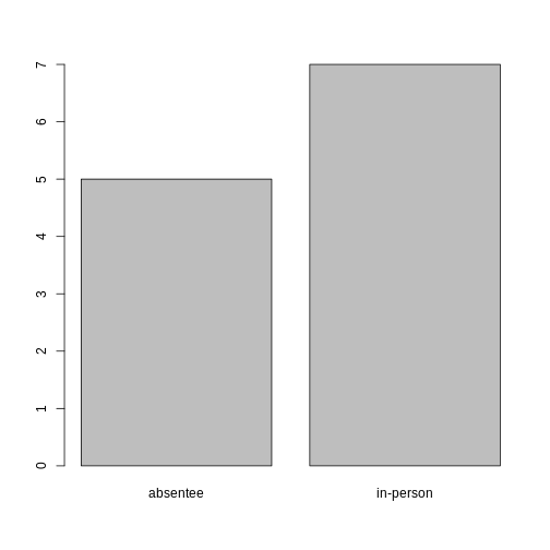
Looking at the plot compared to the output of the vector, we can see that in addition to “absentee”s and “in-person”s, there are some people for whom their ballot type was not noted. Consequently, these people do not appear on the plot! Let’s encode them differently so they can be counted and visualized in our plot.
R
#recreates the data
ballotData <- c("in-person", "in-person", "in-person", "in-person", "in-person", "in-person", "in-person", "absentee", "absentee", "absentee", "absentee", "absentee", NA, NA)

#replace the missing data with "undetermined"
ballotData[is.na(ballotData)] <- "undetermined"

#convert it into a factor
ballotData <- as.factor(ballotData)

#prints out the data (as a vector)
ballotData
OUTPUT
[1] in-person in-person in-person in-person in-person
[6] in-person in-person absentee absentee absentee
[11] absentee absentee undetermined undetermined
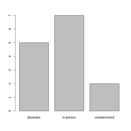
Levels: absentee in-person undeterminedR
#bar plot of the number of cases per ballot type:
plot(ballotData)
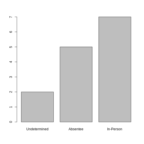
Exercise
- Rename the levels of the factor to be in title case: “Absentee”,“In-Person”, and “Undetermined”.
2, Now that we have renamed the factor level to “Undetermined”, can you recreate the bar plot such that “Undetermined” is first (before “Absentee”)?
R
#part 1:
ballotData <- fct_recode(ballotData,
                         "Absentee" = "absentee",
                         "In-Person" = "in-person",
                         "Undetermined" = "undetermined")

#part 2:
ballotData <- factor(ballotData,
                     levels = c("Undetermined", "Absentee", "In-Person"))
plot(ballotData)
Formatting Dates
Recall our coverage of dates in “Intro to R”. A best practice for
dealing with date data is to ensure that each component of your date is
available as a separate variable. In our dataset, we have a column
checkin_time which contains information about theyear,
month, day, hour, minute, and second that the person that submitted the
ballot arrived in the building. Let’s convert those dates into six
separate columns.
R
str(data)
We are going to use the package
lubridate, , which is included in the
tidyverse installation and should be
loaded by default. However, if we deal with older versions of tidyverse
(2022 and earlier), we can manually load it by typing
library(lubridate).
If necessary, start by loading the required package:
R
library(lubridate)
The lubridate function ymd_hms() takes a vector
representing year, month, day, hour, minutes, and seconds and converts
it to a Date vector.
Let’s extract our checkin_time column and inspect the
structure:
R
times <- data$checkin_time
str(times)
OUTPUT
POSIXct[1:352112], format: "2018-11-06 07:02:36" "2018-11-06 07:04:09" "2018-11-06 07:05:13" ...When we imported the data in R, read_csv() recognized
that this column contained date information. We can now use the
day(), month(), year(),
hour(), minute(), and second()
functions to extract this information from the date, and create new
columns in our data frame to store it:
R
data$day <- day(times)
data$month <- month(times)
data$year <- year(times)
data$hour <- hour(times)
data$minute <- minute(times)
data$seconds <- second(times)

data
OUTPUT
# A tibble: 352,112 × 11
   checkin_id     checkin_time        location precinct device   day month  year
   <chr>          <dttm>              <chr>       <dbl> <chr>  <int> <dbl> <dbl>
 1 CHECKIN_000001 2018-11-06 07:02:36 LOCATIO…     2866 DEVIC…     6    11  2018
 2 CHECKIN_000002 2018-11-06 07:04:09 LOCATIO…     2866 DEVIC…     6    11  2018
 3 CHECKIN_000003 2018-11-06 07:05:13 LOCATIO…     2866 DEVIC…     6    11  2018
 4 CHECKIN_000004 2018-11-06 07:06:26 LOCATIO…     2866 DEVIC…     6    11  2018
 5 CHECKIN_000005 2018-11-06 07:08:08 LOCATIO…     2866 DEVIC…     6    11  2018
 6 CHECKIN_000006 2018-11-06 07:08:32 LOCATIO…     2866 DEVIC…     6    11  2018
 7 CHECKIN_000007 2018-11-06 07:09:36 LOCATIO…     2866 DEVIC…     6    11  2018
 8 CHECKIN_000008 2018-11-06 07:10:18 LOCATIO…     2866 DEVIC…     6    11  2018
 9 CHECKIN_000009 2018-11-06 07:12:57 LOCATIO…     2866 DEVIC…     6    11  2018
10 CHECKIN_000010 2018-11-06 07:13:41 LOCATIO…     2866 DEVIC…     6    11  2018
# ℹ 352,102 more rows
# ℹ 3 more variables: hour <int>, minute <int>, seconds <dbl>
Notice the six new columns at the end of our data frame.
In our example above, the checkin_time column was read
in correctly as a Date variable but generally that is not
the case. Date columns are often read in as character
variables and, similarly to how you can convert character variables to
dates using the as_date() function, columns can be
converted to the appropriate Date/POSIXctformat.
Let’s say we have a generic tibble of IDs and character dates, as configured:
R
data2 <- tibble(
  ID = c("001", "002", "003"),
  Date = c("01/05/2025", "04/23/2024", "12/25/1987")
)

data2
OUTPUT
# A tibble: 3 × 2
  ID    Date
  <chr> <chr>
1 001   01/05/2025
2 002   04/23/2024
3 003   12/25/1987
As you can see, the Date column is stored as characters.
We can easily convert this to a date type by doing one of the
following:
R
#option 1: base R (as.Date)
data2$Date1 <- as.Date(data2$Date, format = "%m/%d/%Y")

#option 2: lubridate (mdy)
data2$Date2 <- mdy(data2$Date)

data2
OUTPUT
# A tibble: 3 × 4
  ID    Date       Date1      Date2
  <chr> <chr>      <date>     <date>
1 001   01/05/2025 2025-01-05 2025-01-05
2 002   04/23/2024 2024-04-23 2024-04-23
3 003   12/25/1987 1987-12-25 1987-12-25
Date1 and Date2 store the exact same data!
Lubridate is preferred to base R, but either function can be used.
Key Points
- Use read_csv to read tabular data in R.
- Access rows and columns in a tibble in R.
- Use factors to represent categorical data in R.
- Use datetime to represent data in R.
- Output a changed dataset to CSV in R.